How To Complete The Data After Imputation R

Past Chaitanya Sagar, Perceptive Analytics.

Missing Data in Analysis

At times while working on data, one may come across missing values which can potentially pb a model off-target. Handling missing values is one of the worst nightmares a information analyst dreams of. If the dataset is very large and the number of missing values in the data are very minor (typically less than 5% as the instance may be), the values can be ignored and analysis can exist performed on the rest of the information. Sometimes, the number of values are likewise big. Withal, in situations, a wise annotator 'imputes' the missing values instead of dropping them from the data.

What Are Missing Values

Think of a scenario when you are collecting a survey data where volunteers fill their personal details in a grade. For someone who is married, i'southward marital status will be 'married' and one will be able to fill the proper noun of one's spouse and children (if whatever). For those who are single, their marital status volition be 'unmarried' or 'unmarried'.

At this indicate the name of their spouse and children volition exist missing values because they will leave those fields blank. This is just one genuine case. There can exist cases as unproblematic every bit someone simply forgetting to notation down values in the relevant fields or every bit complex every bit incorrect values filled in (such equally a name in place of engagement of birth or negative age). At that place are then many types of missing values that nosotros first need to notice out which form of missing values we are dealing with.

Types of Missing Values

Missing values are typically classified into 3 types - MCAR, MAR, and NMAR.

MCAR stands for Missing Completely At Random and is the rarest type of missing values when in that location is no cause to the missingness. In other words, the missing values are unrelated to whatever feature, just equally the name suggests.

MAR stands for Missing At Random and implies that the values which are missing tin be completely explained by the data we already have. For example, there may exist a case that Males are less likely to fill a survey related to depression regardless of how depressed they are. Categorizing missing values every bit MAR actually comes from making an assumption well-nigh the data and there is no way to prove whether the missing values are MAR. Whenever the missing values are categorized as MAR or MCAR and are as well large in number then they can be safely ignored.

If the missing values are not MAR or MCAR and so they autumn into the tertiary category of missing values known every bit Not Missing At Random, otherwise abbreviated as NMAR. The first example beingness talked about here is NMAR category of data. The fact that a person's spouse proper noun is missing can mean that the person is either non married or the person did not fill the name willingly. Thus, the value is missing not out of randomness and we may or may not know which case the person lies in. Who knows, the marital status of the person may also be missing!

If the analyst makes the error of ignoring all the data with spouse name missing he may stop up analyzing only on data containing married people and atomic number 82 to insights which are non completely useful every bit they exercise not represent the entire population. Hence, NMAR values necessarily need to be dealt with.

Imputing Missing Values

Data without missing values can be summarized past some statistical measures such equally mean and variance. Hence, i of the easiest means to fill up or 'impute' missing values is to fill them in such a fashion that some of these measures exercise not change. For numerical data, one can impute with the mean of the data so that the overall mean does not change.

In this process, however, the variance decreases and changes. In some cases such as in time serial, 1 takes a moving window and replaces missing values with the mean of all existing values in that window. This method is also known every bit method of moving averages.

For non-numerical information, 'imputing' with way is a mutual choice. Had we predict the likely value for non-numerical data, nosotros volition naturally predict the value which occurs nearly of the time (which is the fashion) and is elementary to impute.

In some cases, the values are imputed with zeros or very large values and so that they can be differentiated from the rest of the data. Similarly, imputing a missing value with something that falls outside the range of values is also a choice.

An example for this will exist imputing historic period with -i so that it can be treated separately. However, these are used just for quick analysis. For models which are meant to generate concern insights, missing values need to be taken care of in reasonable ways. This volition as well aid 1 in filling with more than reasonable data to train models.

More R Packages for Missing Values

In R, in that location are a lot of packages available for imputing missing values - the popular ones existence Hmisc, missForest, Amelia and mice. The mice package which is an abbreviation for Multivariate Imputations via Chained Equations is ane of the fastest and probably a golden standard for imputing values. Permit us wait at how it works in R.

Using the mice Parcel - Dos and Don'ts

The mice packet in R is used to impute MAR values simply. Equally the name suggests, mice uses multivariate imputations to estimate the missing values. Using multiple imputations helps in resolving the uncertainty for the missingness.

The package provides four different methods to impute values with the default model existence linear regression for continuous variables and logistic regression for chiselled variables. The idea is simple!

If any variable contains missing values, the packet regresses it over the other variables and predicts the missing values. Some of the available models in mice package are:

PMM (Predictive Mean Matching) - suitable for numeric variables
logreg(Logistic Regression) - suitable for chiselled variables with 2 levels
polyreg(Bayesian polytomous regression) - suitable for categorical variables with more than than or equal to two levels
Proportional odds model - suitable for ordered categorical variables with more than or equal to two levels

In R, I will apply the NHANES dataset (National Health and Nutrition Examination Survey data by the US National Center for Health Statistics). We outset load the required libraries for the session:

#Loading the mice package library(mice)  #Loading the post-obit packet for looking at the missing values library(VIM) library(lattice) data(nhanes)

The NHANES data is a small dataset of 25 observations, each having 4 features - age, bmi, hypertension status and cholesterol level. Let'southward run into how the data looks like:

# First await at the data str(nhanes)  'data.frame':	25 obs. of  4 variables:  $ age: num  1 two 1 3 ane iii one i 2 2 ...  $ bmi: num  NA 22.7 NA NA 20.4 NA 22.5 xxx.i 22 NA ...  $ hyp: num  NA 1 ane NA 1 NA one i 1 NA ...  $ chl: num  NA 187 187 NA 113 184 118 187 238 NA ...

The str function shows us that bmi, hyp and chl has NA values which means missing values. The age variable does not happen to have whatever missing values. The age values are only i, 2 and 3 which signal the age bands 20-39, 40-59 and 60+ respectively. These values are ameliorate represented as factors rather than numeric. Allow'southward catechumen them:

#Catechumen Age to factor nhanes$historic period=every bit.factor(nhanes$historic period)

It'southward fourth dimension to get our hands dirty. Let's notice the missing values in the data offset. The mice packet provides a function dr..blueprint() for this:

#understand the missing value pattern md.pattern(nhanes)   	  age	hyp 	bmi 	chl    13   	1   	1   	1   	one  	0  1   	i   	1   	0   	1  	one  three   	1   	1   	1   	0  	one  1   	1   	0   	0   	one  	two  7   	1   	0   	0   	0  	iii      	0   	8   	9  	ten 	27

The output can be understood equally follows. ane's and 0'south under each variable represent their presence and missing state respectively. The numbers before the commencement variable (13,1,3,ane,seven here) represent the number of rows. For example, there are 3 cases where chl is missing and all other values are present. Similarly, at that place are 7 cases where we but take historic period variable and all others are missing. In this way, there are v different missingness patterns. The VIM parcel is a very useful package to visualize these missing values.

#plot the missing values nhanes_miss = aggr(nhanes, col=mdc(i:2), numbers=Truthful, sortVars=True, labels=names(nhanes), cex.axis=.7, gap=3, ylab=c("Proportion of missingness","Missingness Pattern"))

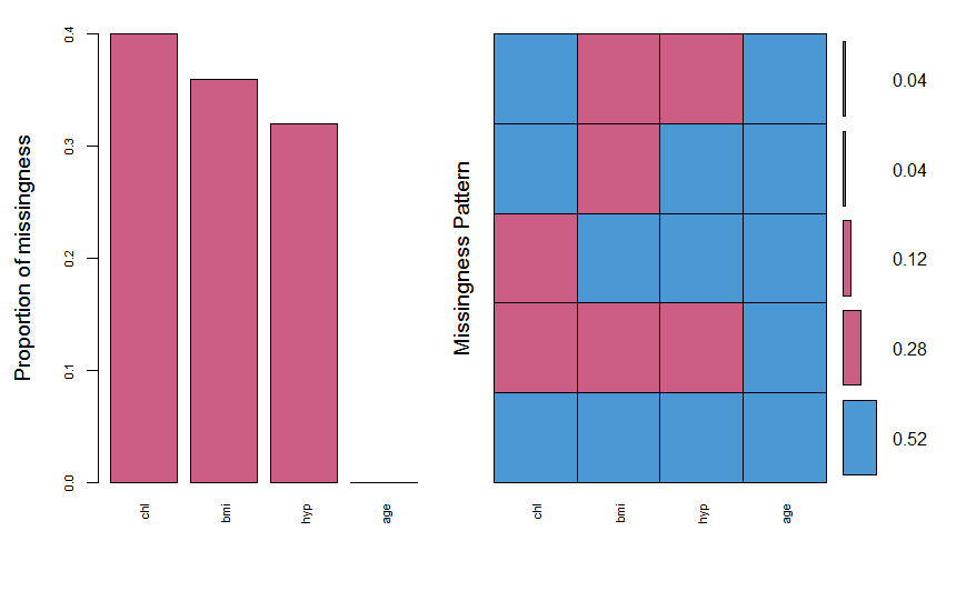
Nosotros meet that the variables accept missing values from xxx-40%. It also shows the different types of missing patterns and their ratios. The next thing is to describe a margin plot which is also office of VIM packet.

#Cartoon margin plot marginplot(nhanes[, c("chl", "bmi")], col = mdc(ane:2), cex.numbers = 1.2, pch = nineteen)

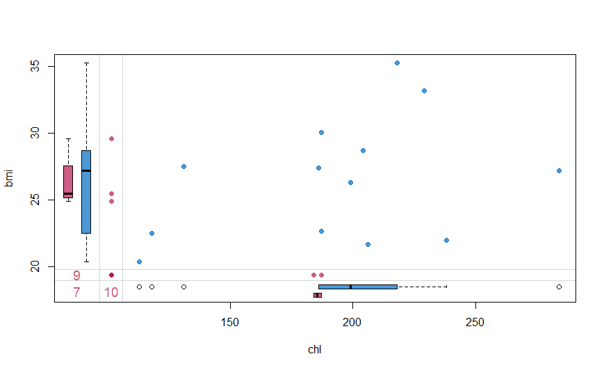
The margin plot, plots two features at a fourth dimension. The ruby plot indicates distribution of one characteristic when it is missing while the blue box is the distribution of all others when the feature is present. This plot is useful to understand if the missing values are MCAR. For MCAR values, the crimson and blue boxes will exist identical.

Let'due south effort to use mice package and impute the chl values:

#Imputing missing values using mice mice_imputes = mice(nhanes, m=5, maxit = xl)

I have used three parameters for the parcel. The outset is the dataset, the second is the number of times the model should run. I have used the default value of 5 here. This means that I now have 5 imputed datasets. Every dataset was created after a maximum of 40 iterations which is indicated by "maxit" parameter.

Allow's meet the methods used for imputing:

#What methods were used for imputing mice_imputes$method    historic period   bmi   	hyp   	chl     "" 	"pmm" 	"pmm" 	"pmm"

Since all the variables were numeric, the packet used pmm for all features. Let's look at our imputed values for chl

            1   	2   	3   	4   	5 1  	187 	118 	238 	187 	187 four  	186 	204 	218 	199 	204 10 	187 	186 	199 	204 	284 11 	131 	131 	199 	238 	199 12 	131 	187 	229 	204 	186 xv 	131 	238 	187 	187 	187 16 	118 	199 	118 	131 	187 20 	206 	184 	184 	218 	229 21 	131 	118 	113 	113 	131 24 	199 	218 	206 	218 	206

We have ten missing values in row numbers indicated by the first column. The next five columns show the imputed values. In our missing data, nosotros have to decide which dataset to use to fill up missing values. This is and so passed to complete() part. I volition impute the missing values from the fifth dataset in this example

#Imputed dataset Imputed_data=complete(mice_imputes,five)

Goodness of fit

The values are imputed but how expert were they? The xyplot() and densityplot() functions come into picture and help us verify our imputations

#Plotting and comparing values with xyplot() xyplot(mice_imputes, bmi ~ chl | .imp, pch = 20, cex = 1.iv)

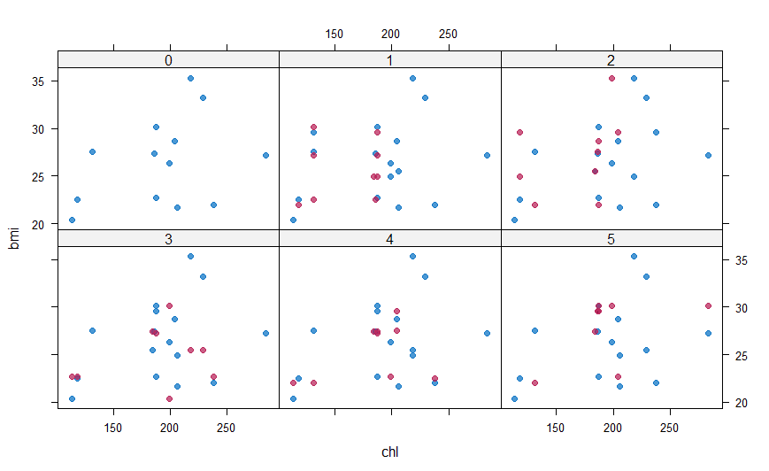
Here again, the blue ones are the observed data and red ones are imputed data. The red points should ideally be similar to the bluish ones so that the imputed values are like. We tin can also await at the density plot of the data.

#make a density plot densityplot(mice_imputes)

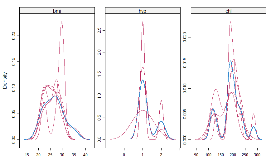
Just as it was for the xyplot(), the ruby imputed values should be like to the blue imputed values for them to exist MAR here.

Summary - Modelling with mice

Imputing missing values is only the starting step in data processing. Using the mice package, I created five imputed datasets just used only one to fill the missing values. Since all of them were imputed differently, a robust model can be developed if 1 uses all the five imputed datasets for modelling. With this in mind, I tin use two functions - with() and pool().

The with() role can be used to fit a model on all the datasets merely as in the post-obit example of linear model

#fit a linear model on all datasets together lm_5_model=with(mice_imputes,lm(chl~historic period+bmi+hyp))  #Use the pool() function to combine the results of all the models combo_5_model=pool(lm_5_model)

The mice package is a very fast and useful packet for imputing missing values. It can impute well-nigh whatever type of data and do it multiple times to provide robustness. We tin can too utilize with() and pool() functions which are helpful in modelling over all the imputed datasets together, making this package pack a punch for dealing with MAR values.

The full code used in this article is provided here.

Bio: Chaitanya Sagar is the Founder and CEO of Perceptive Analytics. Perceptive Analytics has been chosen as 1 of the acme 10 analytics companies to watch out for by Analytics India Magazine. Information technology works on Marketing Analytics for eastward-commerce, Retail and Pharma companies.

Related: