How To Generate A Data Table From One Input Cell Google Sheets

In Microsoft Excel, information tables are office of a suite of commands known equally What-If analysis tools. When you construct and analyze information tables, you are doing what-if assay.

What-if assay is the process of changing the values in cells to meet how those changes will affect the consequence of formulas on the worksheet. For case, y'all can use a information table to vary the interest rate and term length for a loan—to evaluate potential monthly payment amounts.

Types of what-if analysis

There are three types of what-if analysis tools in Excel: scenarios, data tables, and goal-seek. Scenarios and information tables employ sets of input values to calculates possible results. Goal-seek is distinctly different, it uses a single result and calculates possible input values that would produce that result.

Like scenarios, data tables help you explore a fix of possible outcomes. Dissimilar scenarios, information tables evidence you all the outcomes in one tabular array on one worksheet. Using information tables makes it easy to examine a range of possibilities at a glance. Considering yous focus on simply 1 or ii variables, results are like shooting fish in a barrel to read and share in tabular form.

A data table cannot accommodate more than than 2 variables. If you want to analyze more than than two variables, you should instead utilize scenarios. Although it is limited to only ane or two variables (1 for the row input cell and one for the cavalcade input jail cell), a data tabular array can include as many different variable values every bit y'all want. A scenario can have a maximum of 32 dissimilar values, but you tin create as many scenarios as you want.

Learn more than in the commodity, Introduction to What-If Analysis.

Create either one-variable or two-variable data tables, depending on the number of variables and formulas that you lot need to test.

One-variable data tables

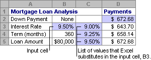
Utilise a i-variable data table if y'all want to encounter how different values of 1 variable in one or more formulas will change the results of those formulas. For instance, yous can use a one-variable information table to encounter how different interest rates affect a monthly mortgage payment past using the PMT function. You enter the variable values in one column or row, and the outcomes are displayed in an adjacent column or row.

In the following analogy, cell D2 contains the payment formula, =PMT(B3/12,B4,-B5), which refers to the input jail cell B3.

Data table with one variable

Two-variable information tables

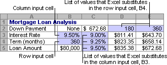
Use a two-variable data table to see how different values of two variables in ane formula will change the results of that formula. For example, y'all can utilize a two-variable data tabular array to come across how different combinations of involvement rates and loan terms volition touch on a monthly mortgage payment.

In the following analogy, cell C2 contains the payment formula, =PMT(B3/12,B4,-B5), which uses two input cells, B3 and B4.

Data table with two variables

Data table calculations

Whenever a worksheet recalculates, whatever data tables will also recalculate—even if there has been no change to the data. To speed up calculation of a worksheet that contains a data table, y'all can change the Adding options to automatically recalculate the worksheet but not the information tables. To learn more, come across the department Speed up calculation in a worksheet that contains data tables.

A ane-variable data table contain its input values either in a single column (cavalcade-oriented), or across a row (row-oriented). Whatsoever formula in a 1-variable data tabular array must refer to only one input cell.

Follow these steps:

Type the listing of values that you lot want to substitute in the input jail cell—either down ane column or across ane row. Exit a few empty rows and columns on either side of the values.
Do one of the following:
- If the data table is cavalcade-oriented (your variable values are in a column), type the formula in the cell one row in a higher place and one cell to the right of the column of values. This ane-variable data table is column-oriented, and the formula is independent in cell D2.
  
  If you desire to examine the effects of diverse values on other formulas, enter the additional formulas in cells to the right of the first formula.
- If the information table is row-oriented (your variable values are in a row), type the formula in the jail cell one column to the left of the first value and one cell below the row of values.
  
  If y'all want to examine the effects of various values on other formulas, enter the additional formulas in cells below the first formula.
Select the range of cells that contains the formulas and values that you lot want to substitute. In the figure higher up, this range is C2:D5.
On the Information tab, click What-If Analysis >Information Tabular array (in the Data Tools group or Forecast group of Excel 2016).
Do one of the following:
- If the data table is column-oriented, enter the cell reference for the input cell in the Column input jail cell field. In the figure in a higher place, the input jail cell is B3.
- If the data table is row-oriented, enter the cell reference for the input cell in the Row input cell field.
  
  Note:Later on you create your data table, you might want to change the format of the consequence cells. In the figure, the issue cells are formatted as currency.

Formulas that are used in a one-variable information table must refer to the same input cell.

Follow these steps

Do either of these:
- If the data tabular array is column-oriented, enter the new formula in a blank prison cell to the right of an existing formula in the top row of the data table.
- If the data table is row-oriented, enter the new formula in a empty cell beneath an existing formula in the first column of the data tabular array.
Select the range of cells that contains the data table and the new formula.
On the Data tab, click What-If Assay >Data Table (in the Data Tools group or Forecast group of Excel 2016).
Practise either of the post-obit:
- If the data table is column-oriented, enter the cell reference for the input cell in the Column input cell box.
- If the data table is row-oriented, enter the jail cell reference for the input prison cell in the Row input prison cell box.

A two-variable data tabular array uses a formula that contains 2 lists of input values. The formula must refer to two different input cells.

Follow these steps:

In a cell on the worksheet, enter the formula that refers to the two input cells.

In the following example—in which the formula starting values are entered in cells B3, B4, and B5, yous type the formula =PMT(B3/12,B4,-B5) in cell C2.
Type one list of input values in the aforementioned cavalcade, below the formula.

In this case, type the different interest rates in cells C3, C4, and C5.
Enter the second list in the aforementioned row as the formula—to its right.

Blazon the loan terms (in months) in cells D2 and E2.
Select the range of cells that contains the formula (C2), both the row and column of values (C3:C5 and D2:E2), and the cells in which you want the calculated values (D3:E5).

In this case, select the range C2:E5.
On the Data tab, in the Data Tools group or Forecast group (in Excel 2016), click What-If Analysis >Data Table (in the Data Tools grouping or Forecast grouping of Excel 2016).
In the Row input cell field, enter the reference to the input cell for the input values in the row.
Type jail cell B4 in the Row input prison cell box.
In the Column input cell field, enter the reference to the input cell for the input values in the column.
Type B3 in the Column input cell box.
Click OK.

Case of a two-variable information table

A two-variable information table can show how unlike combinations of interest rates and loan terms will impact a monthly mortgage payment. In the figure here, cell C2 contains the payment formula, =PMT(B3/12,B4,-B5), which uses two input cells, B3 and B4.

Data table with two variables

When you set this calculation option, no data-table calculations occur when a recalculation is done on the entire workbook. To manually recalculate your data table, select its formulas and then printing F9.

Follow these steps to improve calculation operation:

Click File > Options > Formulas.
In the Calculation options section, under Summate, click Automated except for data tables.

Tip:Optionally, on the Formulas tab, click the arrow on Calculation Options, then click Automatic Except Data Tables (in the Calculation group).

You lot can use a few other Excel tools to perform what-if analysis if you have specific goals or larger sets of variable data.

Goal Seek

If you know the event to expect from a formula, simply don't know precisely what input value the formula needs to get that result, employ the Goal-Seek characteristic. See the article Use Goal Seek to find the result you want by adjusting an input value.

Excel Solver

You can utilize the Excel Solver add-in to observe the optimal value for a fix of input variables. Solver works with a group of cells (called decision variables, or merely variable cells) that are used in computing the formulas in the objective and constraint cells. Solver adjusts the values in the decision variable cells to satisfy the limits on constraint cells and produce the result y'all want for the objective cell. Learn more than in this article: Define and solve a problem past using Solver.

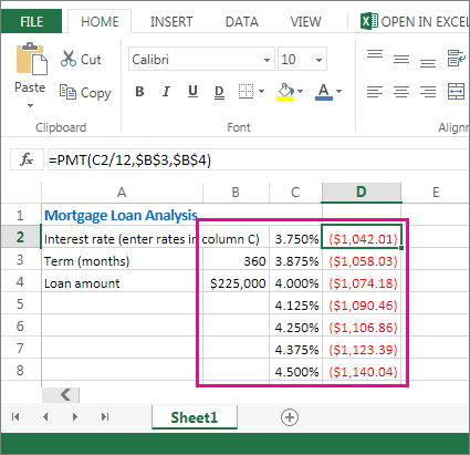
By plugging different numbers into a jail cell, y'all can quickly come upwardly with different answers to a problem. A bully instance is using the PMT role with different interest rates and loan periods (in months) to figure out how much of a loan you can afford for a home or a auto. You lot enter your numbers into a range of cells called a data table.

Here, the data table is the range of cells B2:D8. You lot tin can change the value in B4, the loan corporeality, and the monthly payments in column D automatically update. Using a three.75% interest rate, D2 returns a monthly payment of $ane,042.01 using this formula: =PMT(C2/12,$B$3,$B$iv).

This range of cells, B2:D8, is a data table

You tin can use i or two variables, depending on the number of variables and formulas you want to test.

Use a 1-variable test to see how different values of one variable in a formula will change the results. For example, you can change the interest charge per unit for a monthly mortgage payment by using the PMT function. Y'all enter the variable values (the interest rates) in one column or row, and the outcomes are displayed in a nearby column or row.

In this alive workbook, jail cell D2 contains the payment formula =PMT(C2/12,$B$3,$B$4). Cell B3 is the variable prison cell, where you can plug in a different term length (number of monthly payment periods). In cell D2, the PMT role plugs in the involvement rate 3.75%/12, 360 months, and a $225,000 loan, and calculates a $ane,042.01 monthly payment.

Employ a ii-variable test to see how different values of two variables in a formula will change the results. For case, y'all can test different combinations of interest rates and number of monthly payment periods to calculate a mortgage payment.

In this live workbook, cell C3 contains the payment formula, =PMT($B$3/12,$B$two,B4), which uses ii variable cells, B2 and B3. In cell C2, the PMT function plugs in the interest charge per unit iii.875%/12, 360 months, and a $225,000 loan, and calculates a $1,058.03 monthly payment.